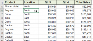
When we are working with many rows of data, it would be time consuming to scroll through all the data to see if there are duplicate rows of information. Luckily for us, Excel has a built-in duplicate remover.
To use this functionality, we need to make sure we select a cell within the data. Excel will select all the data it needs to check, based on the cell you select when you start the process. Also, ensure that your data has column headers, wherever possible, as it will make the process a little easier.

If there are any rows or columns of information missing, it can mess up the process. Missing cells of information here and there will not mess up the process.
Once you are ready to start, follow these steps:
- Click the Data tab
- In the Data Tools group, click Remove Duplicates

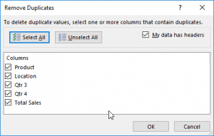
- A dialog box will open with a selection of columns to choose from when comparing for duplicates
 Best practice is to keep all columns selected, as this will only delete true duplicates. However, it is not required to keep all columns selected to run the functionality
 - Once you are ready, click OK. A dialog box will pop-up, stating how many duplicates were deleted

- Click OK again to finish
If for some reason you need to undo this process, click the Undo icon in your Quick Access Toolbar to undo the process. ![]() If you click Save before you undo this process, the duplicate information cannot be brought back.
If you click Save before you undo this process, the duplicate information cannot be brought back.
It is a good practice to clean up your data, before you start printing reports or manipulating your data.


