Freeze Panes in Excel allow users to scroll for information and still have the ability to match column and row headers, allowing a user to not need to constantly scroll back and forth in a worksheet to figure out which information lines up together.
Adding Freeze Panes is very easy in the whole scheme of things, but deciding which option to use, or making sure the table of information is laid out properly, is necessary to ensure that the functionality works properly. Typically, information is laid out with row headers, such as the example below:

or with column headers, as shown below:

or even both.
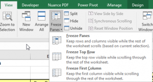
In some cases, there are multiple rows at the top of the worksheet being used for both title and header information, so having the ability to choose where the Freeze Pane is placed is essential. There are three options for Freeze Panes – Freeze Panes, Freeze Top Row, and Freeze First Column. The command for Freeze Panes is located under the View tab in the Windows group. Clicking the drop-down arrow will display the three options.

Freeze Top Row freezes only the top row (row 1) and Freeze First Column freezes only the far left column (column A).  Freeze Panes allows you to set the functionality anywhere within the worksheet.
To use the Freeze Panes option, you must first choose the cell you want the the Freeze Panes based on. Freeze Panes will be added based on this cell and will populate above and to the left of the selected cell, so scrolling will not be available to any columns to the left of the selected cell or above the selected cell. From there, click the Freeze Panes command and the functionality will be added.

For more ways to make Excel work for you, take a training course from AdvantEdge Training & Consulting!