Excel PowerPivot is a tool for managing and visualizing complex data within Excel. It has elements of a database system like Access but also offers Excel features like Pivot Table.
PowerPivot is free with Office 2013, but you may need to enable it. There are directions on how to do so at this link.
Once you’ve enabled PowerPivot, the PowerPivot tab should appear. There are a lot of tools available, but we’ll focus on relating two tables together.
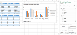
In this example, one table lists individuals with their genders and titles. The other table is the list of miles, sales, and coffee cups. The two tables must hold some column in common in order to create the relationship. In this case, I added a number field for the respondents.
Add to the data model
The first step is to add each table to the data model. To do so, I put my cursor in one of the tables, and clicked on Add to Data Model under the PowerPivot Tab. The system prompted me to format the data in a table. Once I did, it opened a separate PowerPivot window for that table.
I closed the new window and repeated the process for the second table, adding it to the data model as well. Then, in the PowerPivot window that opened, I chose diagram view to set up the relationships.
Creating relationships
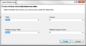
I right clicked on the title for one of the boxes and chose Create Relationship. I then chose the column that was held in common and clicked create. The data model shows this relationship with a line between the two tables.

Using related tables
After creating the relationships. I clicked on the drop down arrow under the PivotTable option to create a pivot chart. Because there is a relationship between the tables I can draw data from both tables.


