The width of columns and height of rows can be adjusted to better fit your data in a few different ways.
Drag the border
![]() Hover your arrow over the border between the column or row labels. Then click and drag the border to widen or narrow the size of each cell. The columns to the right or rows below will adjust to make room for your changes.
Hover your arrow over the border between the column or row labels. Then click and drag the border to widen or narrow the size of each cell. The columns to the right or rows below will adjust to make room for your changes.
Type in your desired width
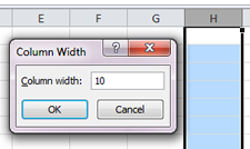
 Right click on the column labels and choose Column Width. Type in a number in the pop up window to change the width of the column. Right click on row labels and choose row width to adjust the width of a row.
Use the format button
The Format button in the cells group under the Home tab can also be used to adjust widths and heights. Simply select the cells that need to be adjusted, then click on the Format button and choose either Row Height or Column Width. Type in your desired number, and the cells will adjust.
Resizing multiple columns at once
You can make several columns or rows the same width or height. Select your desired columns or rows by clicking on the labels while holding down either the shift key or control key. Then use any of the methods described above, and all of the columns will be made the same width or rows the same height.
Adjusting width and height automatically
If several columns or rows in your table need to be adjusted to accommodate your data, Excel can automatically adjust the spreadsheet.
Select all of the columns or all of the rows that contain your data. Then, hover over the border until your arrow becomes a double arrow. Double click on the border, and all of the rows or columns will automatically adjust to fit the data.
To adjust an entire worksheet with both rows and columns, type Control A to select the entire worksheet. Then, double click with a double arrow on any column or row border.


